JSys Screen Shots

Here are some screens shots showing simple models that have been built using JSys. Click on an image to the full sized version.

Simple Harmonic Motion

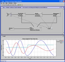
A simulation of simple harmonic motion of a mass on a spring. The simulation features two integrators to solve the differential equation: Acceleration = d²X/dT² = Force/Mass, where X is the displacement from the equilibrium position and T is time . The first integrator determines the velocity from the acceleration and the second determines the position from the velocity. The force is calculated according to Force = -Displacement * SpringConstant.

In the example shown the mass is increased to four times its original value part way throught the simulation resulting in an increase in the period of oscillation..

A Central Heating System

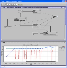
A simple simulation of a central heating system.

There are two loops in the model. One of these (bottom right) models the het loss from the building to the outside. The other (top centre) models the heating, which is controlled by a thermostatic switch.

In the example shown, the outside temperature is changed part way through the run and then the thermostat is set to a higher temperature.

A Manufacturing/Supply System

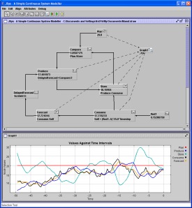
A simple simulation of a manufacturing and supply system. The basic control loop shown in the centre of the diagram controls the production rate to try to keep the amount in the store constant at a planned level. The system includes a simple market forecasting loop to control production rates for observed changes in demand.

In the example, the demand is varied randomly by the consumption calculation in the bottom right of the diagram.

Editing a Node

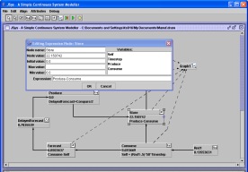
This screenshot shows the parameters being edited in the integrating expression node that represents the store in the manufacturing system example.

The user can edit the mathematical expression, and include variables that represent the time steps, the value of the node itself, and the inputs from all node that feed into this one.

The evaluation of node expressions in JSys makes use of the Java Expression Parser library (JEP). (See: http://www.singularsys.com/jep)

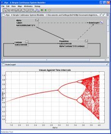
Logistic Map (Showing state space plots.)

This screenshot shows a model implementing the iterated logistic map. The graph plots two model parameters against one-another rather than against time. The model has been arranged so that the value of the parameter Alpha is gradually decreased, starting at just below 4.0, as the model is run. The decrement is arranged so that a large density of points are plotted at the uppoer end of the range, but fewer lower down the range to speed up the calculation.

Pitchfork bifurcations can be clearly seen, and also tangent bifurcations leading to an attractor of period three in the region just above Alpha=3.8.